6 Discrete Random Variables
- Roughly, a random variable assigns a number measuring some quantity of interest to each outcome of a random phenomenon.
- Mathematically, a random variable (RV) \(X\) is a function that takes an outcome in the sample space as input and returns a real number as output
- The random variable itself is typically denoted with a capital letter (\(X\)); possible values of that random variable are denoted with lower case letters (\(x\)).
- Think of the capital letter \(X\) as a label standing in for a formula like “the number of heads in 4 flips of a coin” and
- \(x\) as a dummy variable standing in for a particular value like 3.
- Discrete random variables take at most countably many possible values (e.g., \(0, 1, 2, \ldots\)). They are often counting variables (e.g., the number of Heads in 10 coin flips).
- Continuous random variables can take any real value in some interval (e.g., \([0, 1]\), \([0,\infty)\), \((-\infty, \infty)\).). That is, continuous random variables can take uncountably many different values. Continuous random variables are often measurement variables (e.g., height, weight, income).
- A function of a random variable is also a random variable: if \(X\) is a RV then so is \(g(X)\)
- Sums and products, etc., of random variables defined on the same sample space are random variables. If\(X\) and \(Y\) are RVs defined on the same sample space then so are \(X+Y\), \(X-Y\), \(XY\)
- If the sample space outcomes are represented by rows in a spreadsheet, then random variables correspond to columns.
- Expressions like \(X=x\) or \(\{X=x\}\) represent events: for which outcomes is the value of the random variable \(X\) equal to the value \(x\). (Remember, if the sample space outcomes are represented by rows in a spreadsheet, then an event corresponds to a subset of rows (outcomes) that satisfies some criteria.)
- The (probability) distribution of a collection of random variables identifies the possible values that the random variables can take and their relative likelihoods.
- We will see many ways of describing a distribution, depending on how many random variables are involved and their types (discrete or continuous).
| First roll | Second roll | X | Y |
|---|---|---|---|
| 1 | 1 | ||
| 1 | 2 | ||
| 1 | 3 | ||
| 1 | 4 | ||
| 2 | 1 | ||
| 2 | 2 | ||
| 2 | 3 | ||
| 2 | 4 | ||
| 3 | 1 | ||
| 3 | 2 | ||
| 3 | 3 | ||
| 3 | 4 | ||
| 4 | 1 | ||
| 4 | 2 | ||
| 4 | 3 | ||
| 4 | 4 |
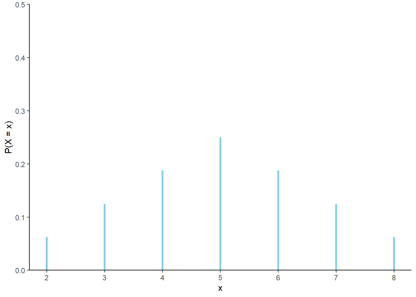
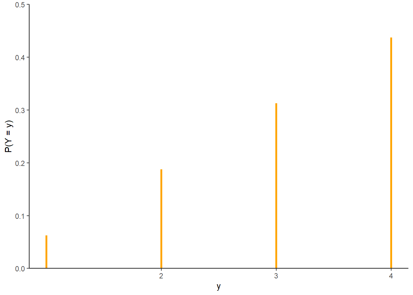
Example 6.1 Roll a four-sided die twice, and record the result of each roll in sequence. Let \(X\) be the sum of the two dice, and let \(Y\) be the larger of the two rolls (or the common value if both rolls are the same). Table 6.1 represents the possible outcomes. Assume the die is fair and the rolls are independent.
- Fill in the values of \(X\) and \(Y\) for each outcome in the table.
- Identify the event \(\{X = 4\}\) and compute its probability. Then interpret the probability both as a long relative frequency and as a relative likelihood.
- Construct a table and plot of \(\text{P}(X = x)\) for each possible value \(x\) of \(X\).
- Construct a table and plot of \(\text{P}(Y = y)\) for each possible value \(y\) of \(Y\).
Example 6.2 Recall the batch testing scenarios from Example 5.2 and Example 5.3. Let \(X\) be the total number of tests required when we test all 8 people in a single batch first, and let \(Y\) be the total number of tests when we split into two batches of 4 people first.
- Identify the distribution of \(X\).
- Identify the distribution of \(Y\).
Example 6.3 The “matching problem” involves \(n\) distincts objects labeled \(1, \ldots, n\) which are placed in \(n\) distinct boxes labeled \(1, \ldots, n\), with exactly one object placed in each box. Suppose the objects are placed in the boxes uniformly at random, so that any possible arrangement is equally likely. Let \(X\) be the number of matches, that is, the number of objects for which their label matches the label of the box in which they are placed.
For example, suppose \(n\) people have a secret Santa gift exchange. Each person puts their name in a hat, the names are well shuffled, and everyone draws a name from the hat (to then purchase a gift for the selected person). Let \(X\) represent the number of people who draw their own name.
Consider the matching problem with \(n=3\). Specify the distribution of \(X\), and interpret it.
6.1 Exercises
Exercise 6.1 Five individuals are interviewing for a single job opening, but only two are qualified for the position. Suppose the individuals are interviewed in a random order, and each individual is only interviewed once, until one of the qualified candidates is interviewed, and then no more candidates are interviewed. Let \(X\) count the number of interviews conducted.
Make a table to represent the distribution of \(X\).
Exercise 6.2 Continuing Example 6.1.
- Describe how you could simulate a single value of \(Y\).
- Construct a spinner (like from a kids game) to represent the distribution of \(Y\).
- Describe another way to simulate a single value of \(Y\).
- Describe how you could use simulation to approximate the distribution of \(Y\).
- Don’t confuse a random variable with its distribution!
- A random variable measures a numerical quantity which depends on the outcome of a random phenomenon
- The distribution of a random variable specifies the long run pattern of variation of values of the random variable over many repetitions of the underlying random phenomenon.
- Any marginal distribution can be represented by a single spinner (like from a kids game).
- In principle, there are always two ways of simulating a value \(x\) of a random variable \(X\).
- Simulate from the probability space. Simulate an outcome \(\omega\) from the underlying probability space and set \(x = X(\omega)\).
- Simulate from the distribution. Construct a spinner corresponding to the distribution of \(X\) and spin it once to generate \(x\).
- The second method requires that the distribution of \(X\) is known. However, as we will see in many examples, it is common to specify the distribution of a random variable directly without defining the underlying probability space.