19 Linear Combinations of Random Variables

In general, the distribution of a sum (or linear combination) of random variables can be difficult to obtain and depends on the joint distribution of the random variables.
But there are some special cases where the distribution of a sum (or linear combination) works out nicely.
And there are shortcut formulas that allow us to find the expected value and variance of a sum (or linear combination) without first finding its distribution.

Example 19.1 At a small hospital, let $X$ be the number of babies born in a 5 day work week and let $Y$ be the number of babies born on a weekend. Then $W = X + Y$ is the total number of babies born in a week. Assume that

$X$ and $Y$ are independent
$X$ has a Poisson(2.1) distribution
$Y$ has a Poisson(0.4) distribution

Table 19.1 displays the marginal distributions of $X$ and $Y$. (The probabilities have been rounded a little.)

Table 19.1: Distributions in Example 19.1

x, y	0	1	2	P(X = x)
0				0.122
1				0.257
2				0.270
3				0.189
4				0.099
5				0.042
6				0.021
P(Y = y)	0.670	0.268	0.062

Create a table for the joint distribution of $X$ and $Y$.
Compute and interpret $\text{P}(W = 0)$.
Compute and interpret $\text{P}(W = 1)$.
Compute and interpret $\text{P}(W = 2)$.
Find the distribution of $W$.
Compute and interpret $\text{E}(W)$. How does it relate to $\text{E}(X)$ and $\text{E}(Y)$?
Compute $\text{Var}(W)$. How does it relate to $\text{Var}(X)$ and $\text{Var}(Y)$?

Poisson aggregation. If $X$ and $Y$ are independent, $X$ has a Poisson($\mu_X$) distribution, and $Y$ has a Poisson($\mu_Y$) distribution, then $X+Y$ has a Poisson($\mu_X+\mu_Y$) distribution.
If component counts are independent and each has a Poisson distribution, then the total count also has a Poisson distribution.

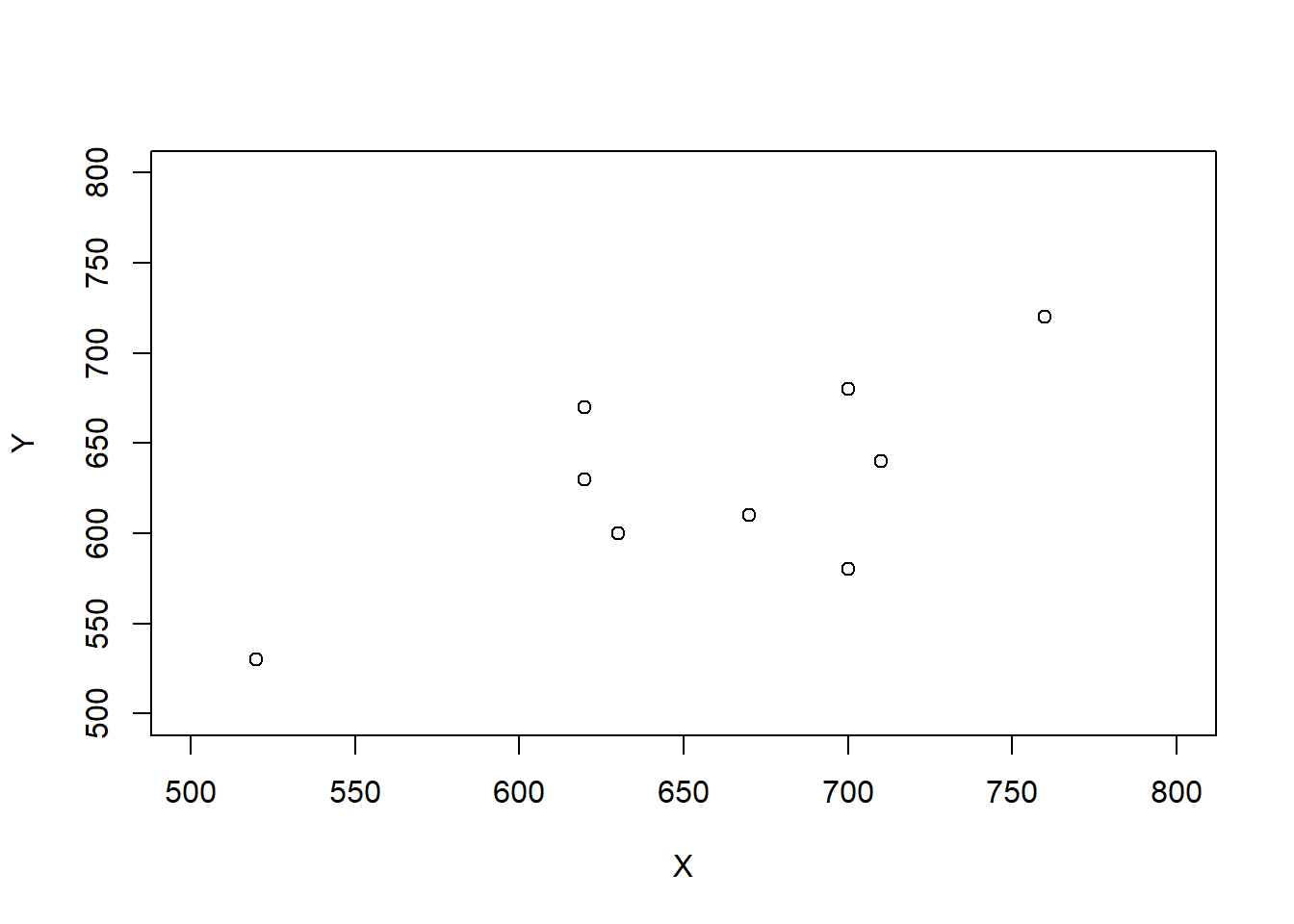
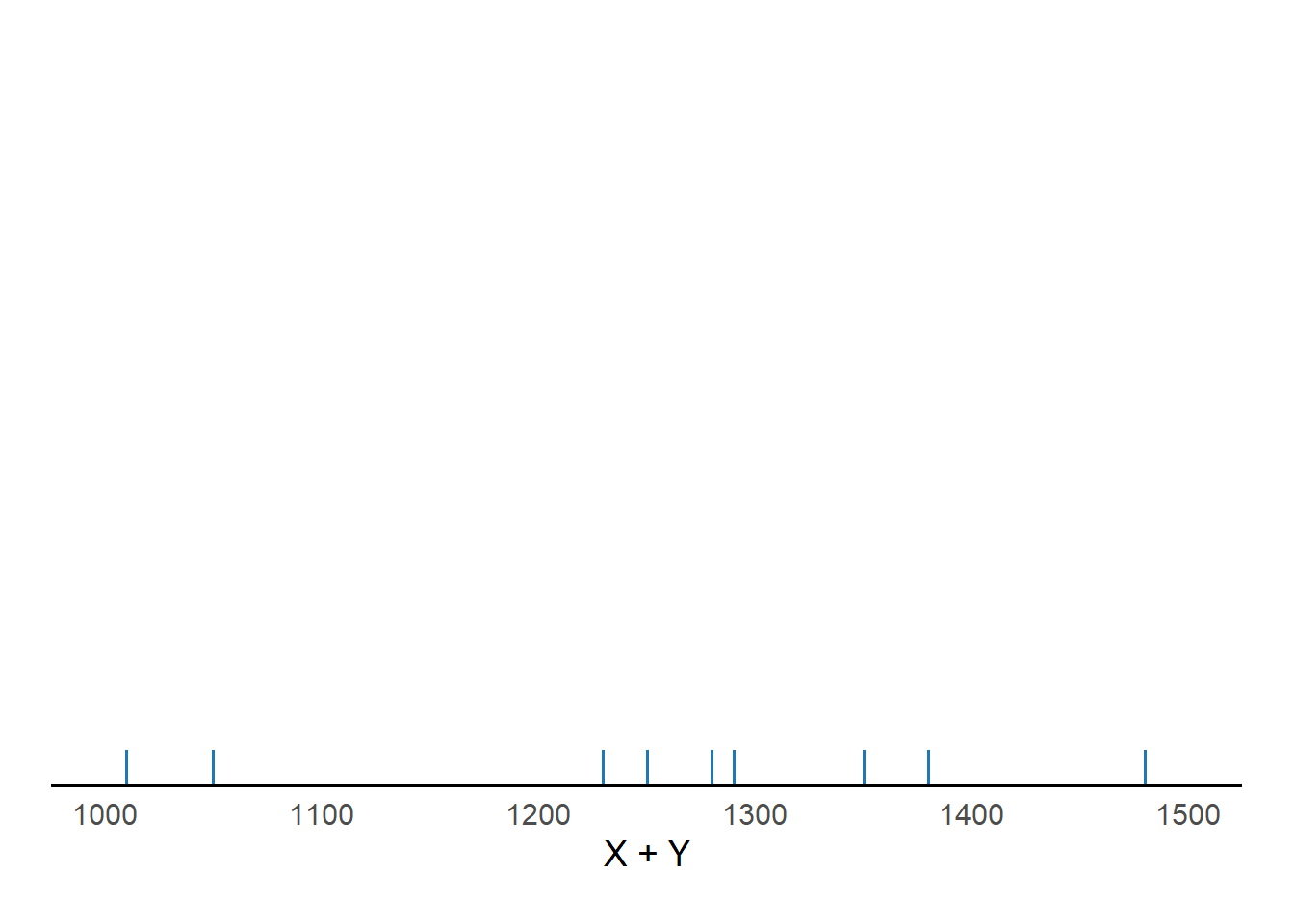
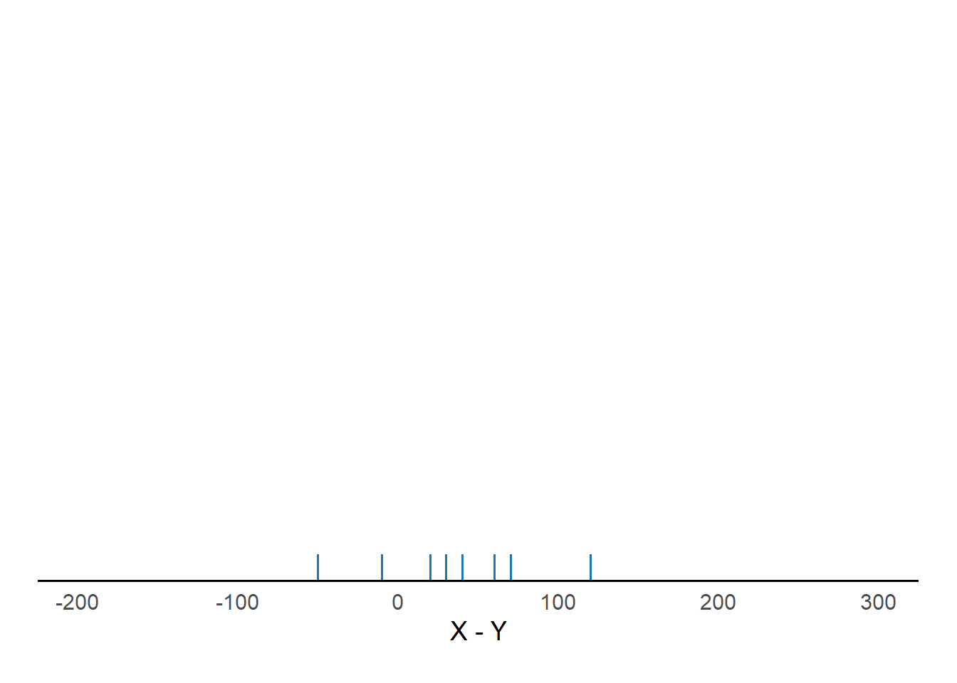
Example 19.2 We’ll illustrate some ideas with a small sample of simulated values. Say we have SAT Math scores ($X$) and Reading scores ($Y$) for 10 students. We’re interested in the sum ($T = X + Y$) and difference (Math minus Reading, $D = X-Y$) of the scores.

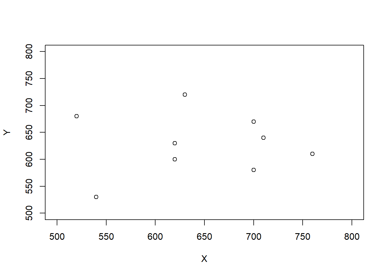
The 10 $X$ values are the same in each scenario, and the 10 $Y$ values are the same in each scenario, but the $(X, Y)$ values are paired in different ways:

Scenario 1: correlation is 0.78
Scenario 2: correlation is about 0 (actually -0.04)
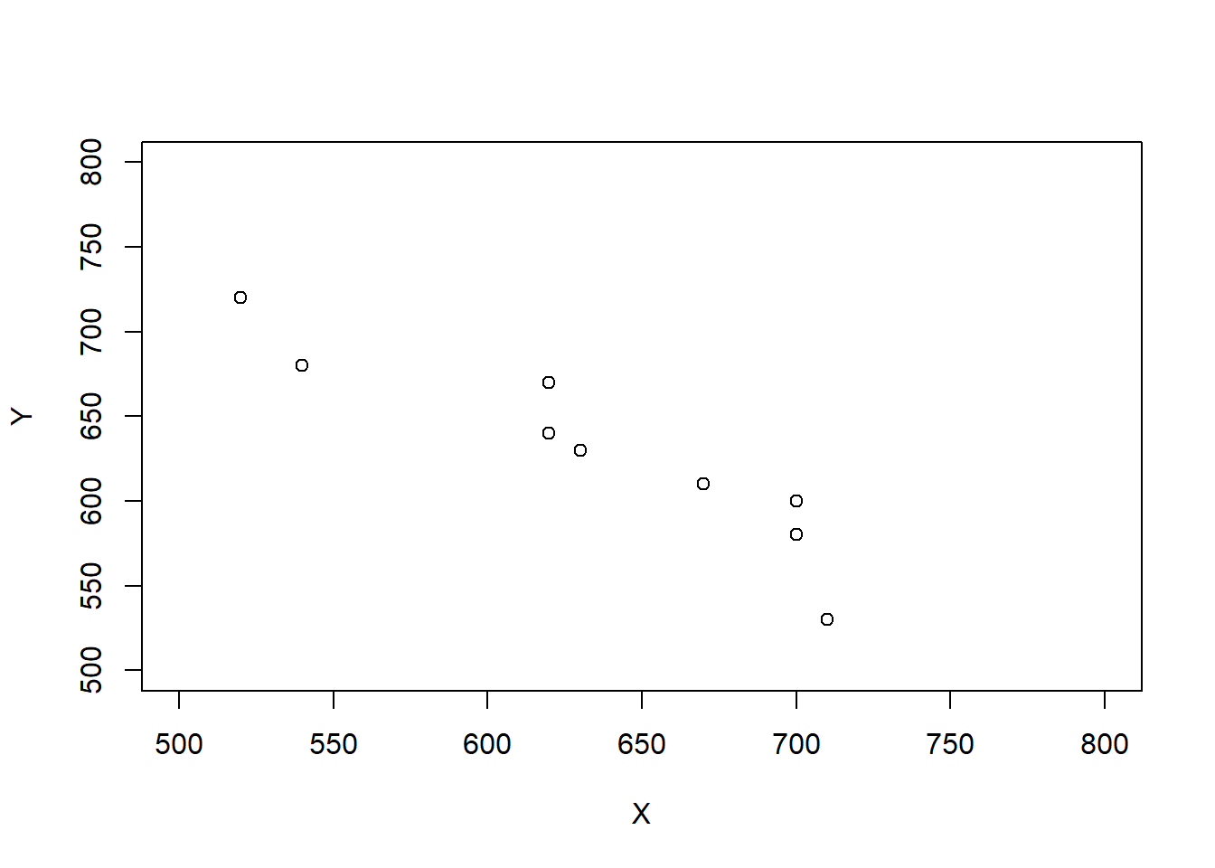
Scenario 3: correlation is -0.94

Table 19.2: Example 19.2 scenario 1, correlation is 0.78

Student	$X$	$Y$	$T$	$D$
1	520	530	1050	-10
2	540	470	1010	70
3	620	670	1290	-50
4	620	630	1250	-10
5	630	600	1230	30
6	670	610	1280	60
7	700	680	1380	20
8	700	580	1280	120
9	710	640	1350	70
10	760	720	1480	40

Mean	647	613	1260	34
SD	72	70	134	47
Corr($X$, $Y$)	0.78

Table 19.3: Example 19.2 scenario 2, correlation is about 0

Student	$X$	$Y$	$T$	$D$
1	520	680	1200	-160
2	540	530	1070	10
3	620	630	1250	-10
4	620	600	1220	20
5	630	720	1350	-90
6	670	470	1140	200
7	700	670	1370	30
8	700	580	1280	120
9	710	640	1350	70
10	760	610	1370	150

Mean	647	613	1260	34
SD	72	70	98	103
Corr($X$, $Y$)	-0.04

Table 19.4: Example 19.2 scenario 3, correlation is -0.94

Student	$X$	$Y$	$T$	$D$
1	520	720	1240	-200
2	540	680	1220	-140
3	620	670	1290	-50
4	620	640	1260	-20
5	630	630	1260	0
6	670	610	1280	60
7	700	600	1300	100
8	700	580	1280	120
9	710	530	1240	180
10	760	470	1230	290

Mean	647	613	1260	34
SD	72	70	26	140
Corr($X$, $Y$)	-0.94

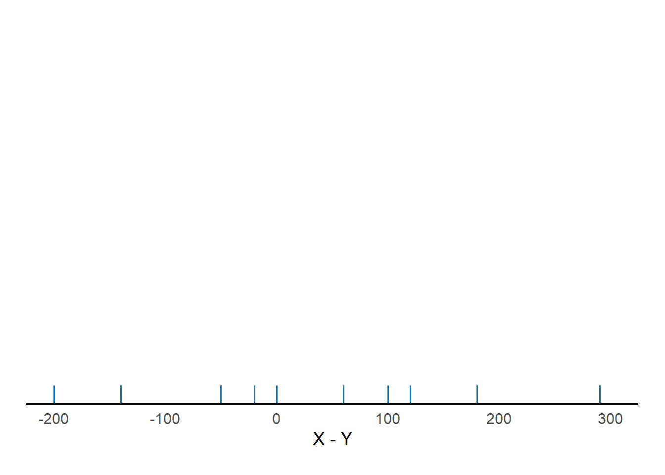
In each scenario:

Compute the mean of total scores.
How does the mean of $X + Y$ relate to the means of $X$ and $Y$?
Compute the mean of the difference in scores (Math – Reading)
How does the mean of $X - Y$ relate to the means of $X$ and $Y$?

Linearity of expected value. For any two random variables $X$ and $Y$, \[\begin{align*} \text{E}(X + Y) & = \text{E}(X) + \text{E}(Y) \end{align*}\]
That is, the expected value of the sum is the sum of expected values, regardless of how the random variables are related.
Therefore, you only need to know the marginal distributions of $X$ and $Y$ to find the expected value of their sum. (But keep in mind that the distribution of $X+Y$ will depend on the joint distribution of $X$ and $Y$.)
Whether in the short run or the long run, \[\begin{align*} \text{Average of $X + Y$ } & = \text{Average of $X$} + \text{Average of $Y$} \end{align*}\] regardless of the joint distribution of $X$ and $Y$.
A linear combination of two random variables $X$ and $Y$ is of the form $aX + bY$ where $a$ and $b$ are non-random constants. Combining properties of linear rescaling with linearity of expected value yields the expected value of a linear combination. \[ \text{E}(aX + bY) = a\text{E}(X)+b\text{E}(Y) \]
For example ($a=1, b=-1$): $\text{E}(X-Y) = \text{E}(X) - \text{E}(Y)$.
Linearity of expected value extends naturally to more than two random variables. \[ \text{E}(a_1X_1 + \cdots + a_nX_n) = a_1\text{E}(X_1) + \cdots + a_n\text{E}(X_n) \]

Example 19.3 Continuing with the three scenarios in Example 19.2.

In each scenario:

Compute the variance of total scores.
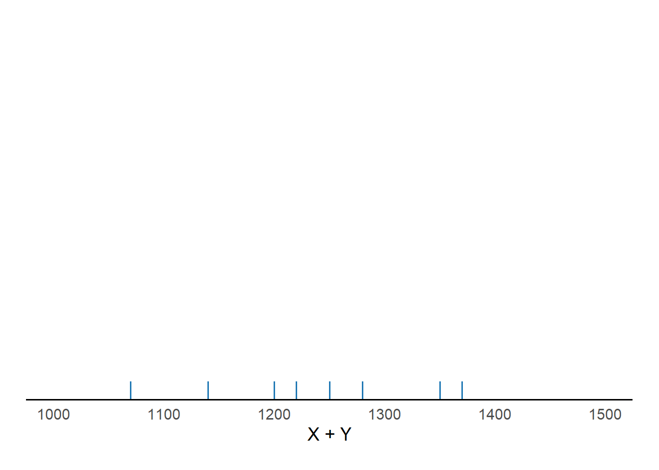
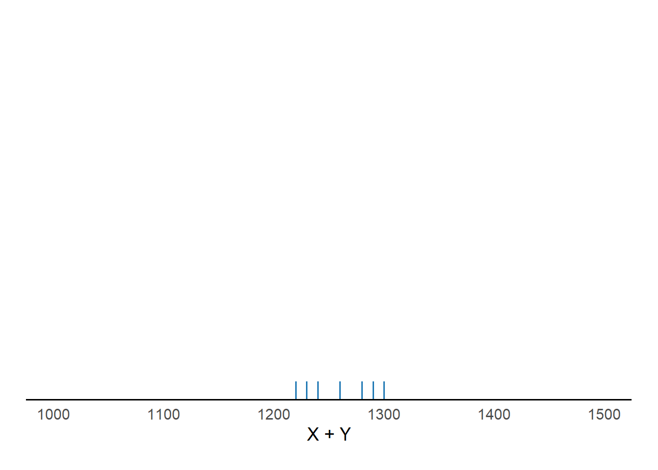
How does correlation affect $\text{Var}(X + Y)$? In which of the three scenarios is $\text{Var}(X + Y)$ the largest? The smallest? Can you explain why? In which scenario is $\text{Var}(X + Y)$ roughly equal to the sum of $\text{Var}(X)$ and $\text{Var}(Y)$?
Compute the variance of the difference in scores (Math - Reading)
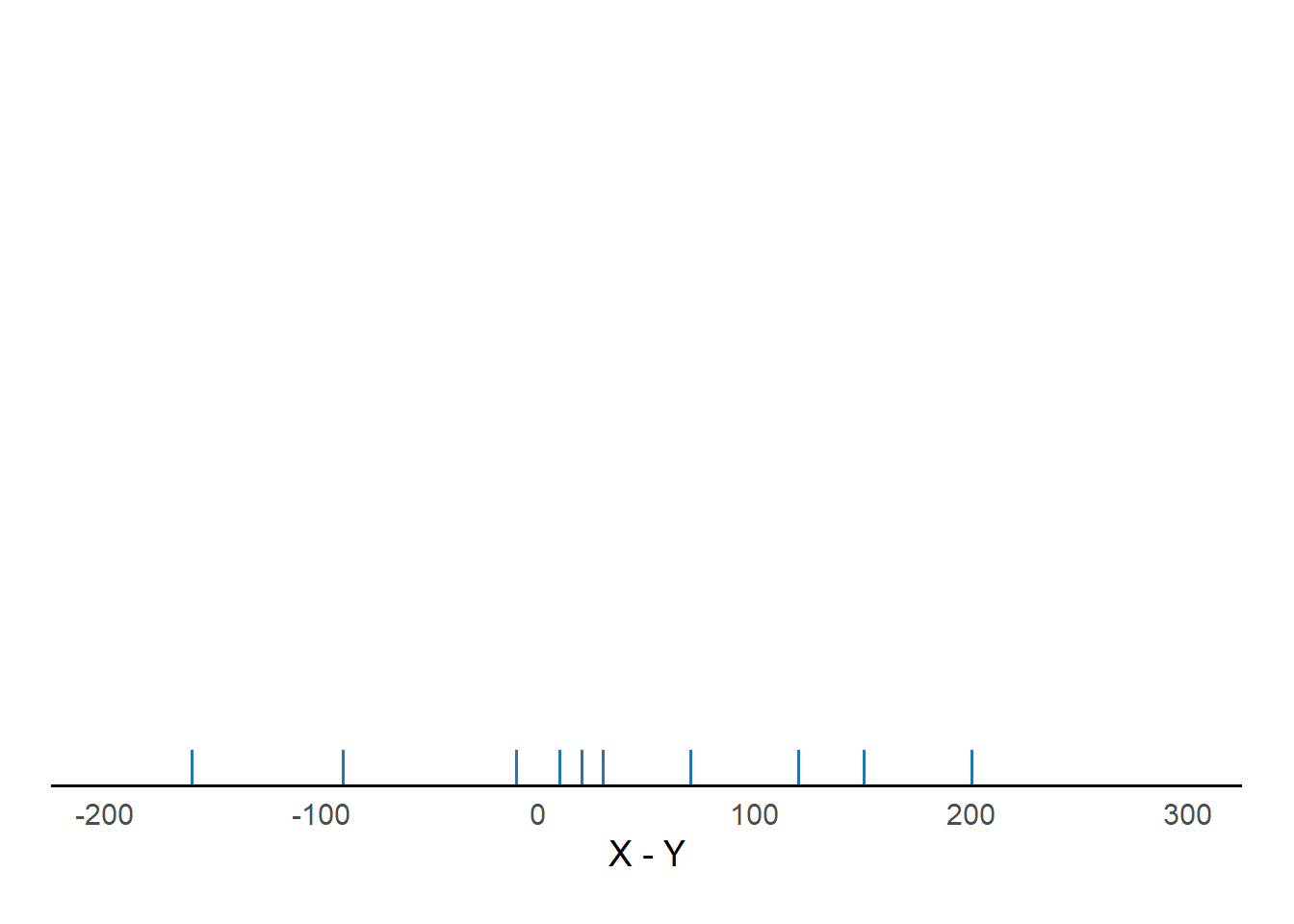
How does correlation affect $\text{Var}(X - Y)$? In which of the three scenarios is $\text{Var}(X - Y)$ the largest? The smallest? Can you explain why? In which scenario is $\text{Var}(X - Y)$ roughly equal to the sum of $\text{Var}(X)$ and $\text{Var}(Y)$?

Variance of sums and differences of random variables \[\begin{align*} \text{Var}(X + Y) & = \text{Var}(X) + \text{Var}(Y) + 2\text{Cov}(X, Y)\\ \text{Var}(X - Y) & = \text{Var}(X) + \text{Var}(Y) - 2\text{Cov}(X, Y) \end{align*}\]
If $X$ and $Y$ are uncorrelated: \[\begin{align*} \text{Var}(X+Y) & = \text{Var}(X) + \text{Var}(Y)\qquad \text{if $X, Y$ are uncorrelated}\\ \text{Var}(X-Y) & = \text{Var}(X) + \text{Var}(Y)\qquad \text{if $X, Y$ are uncorrelated} \end{align*}\]
Variance of linear combinations: If $a, b, c$ are non-random constants and $X$ and $Y$ are random variables then \[ \text{Var}(aX + bY + c) = a^2\text{Var}(X) + b^2\text{Var}(Y) + 2ab\text{Cov}(X, Y) \]

Example 19.4 Let $X$ be the sales of beer and $Y$ the sales of salty snacks in a week at a certain supermarket, measured in thousands of dollars.
Suppose

$\text{E}(X) = 22$, $\text{SD}(X) = 6$
$\text{E}(Y) = 14$, $\text{SD}(Y) = 4$
$\text{Corr}(X, Y) = 0.55$

Compute and intepret $\text{E}(X+Y)$.
Compute and intepret $\text{SD}(X+Y)$.

Example 19.5 Let $X$ be the sales of beer and $Y$ the sales of wine in a week at a certain supermarket, measured in thousands of dollars.
Suppose

$\text{E}(X) = 22$, $\text{SD}(X) = 6$
$\text{E}(Y) = 14$, $\text{SD}(Y) = 4$
$\text{Corr}(X, Y) = -0.55$

Compute and intepret $\text{E}(X+Y)$.
Compute and intepret $\text{SD}(X+Y)$.

19.1 Exercises

Exercise 19.1 Consider a random variable $X$ with $\text{Var}(X)=1$. What is $\text{Var}(2X)$?

Walt says: $\text{SD}(2X) = 2\text{SD}(X)$ so $\text{Var}(2X) = 2^2\text{Var}(X) = 4(1) = 4$.
Jesse says: Variance of a sum is a sum of variances, so $\text{Var}(2X) = \text{Var}(X+X)$ which is equal to $\text{Var}(X)+\text{Var}(X) = 1+1=2$.

Who is correct? Why is the other wrong?

Exercise 19.2 Percent returns for assets $X$, $Y$, and $Z$ follow a joint distribution with

Mean 10 and standard deviation 15 for asset $X$,
Mean 5 and standard deviation 3 for asset $Y$,
Correlation of −0.6 between asset $X$ and asset $Y$
Asset Z yields a constant return of 1 percent.

An investment portfolio has 60% of its funds in asset $X$, 30% in asset $Y$, and 10% in asset $Z$.

Let $R$ be the portfolio return. Express $R$ in terms of $X, Y, Z$.
Compute $\text{E}(R)$.
Compute $\text{Cov}(X, Y)$.
Compute $\text{Cov}(X, Z)$.
Compute $\text{SD}(R)$.