| count | mean | std | min | 25% | 50% | 75% | max | |
|---|---|---|---|---|---|---|---|---|
| treatment | ||||||||
| debridement | 60.0 | 53.983333 | 23.304536 | 10.0 | 40.75 | 52.0 | 76.25 | 97.0 |
| lavage | 60.0 | 56.733333 | 24.150564 | 8.0 | 41.00 | 53.5 | 73.50 | 99.0 |
| placebo | 60.0 | 52.450000 | 25.079146 | 3.0 | 31.00 | 54.0 | 70.25 | 97.0 |
28 Comparing multiple means: ANOVA \(F\) procedures
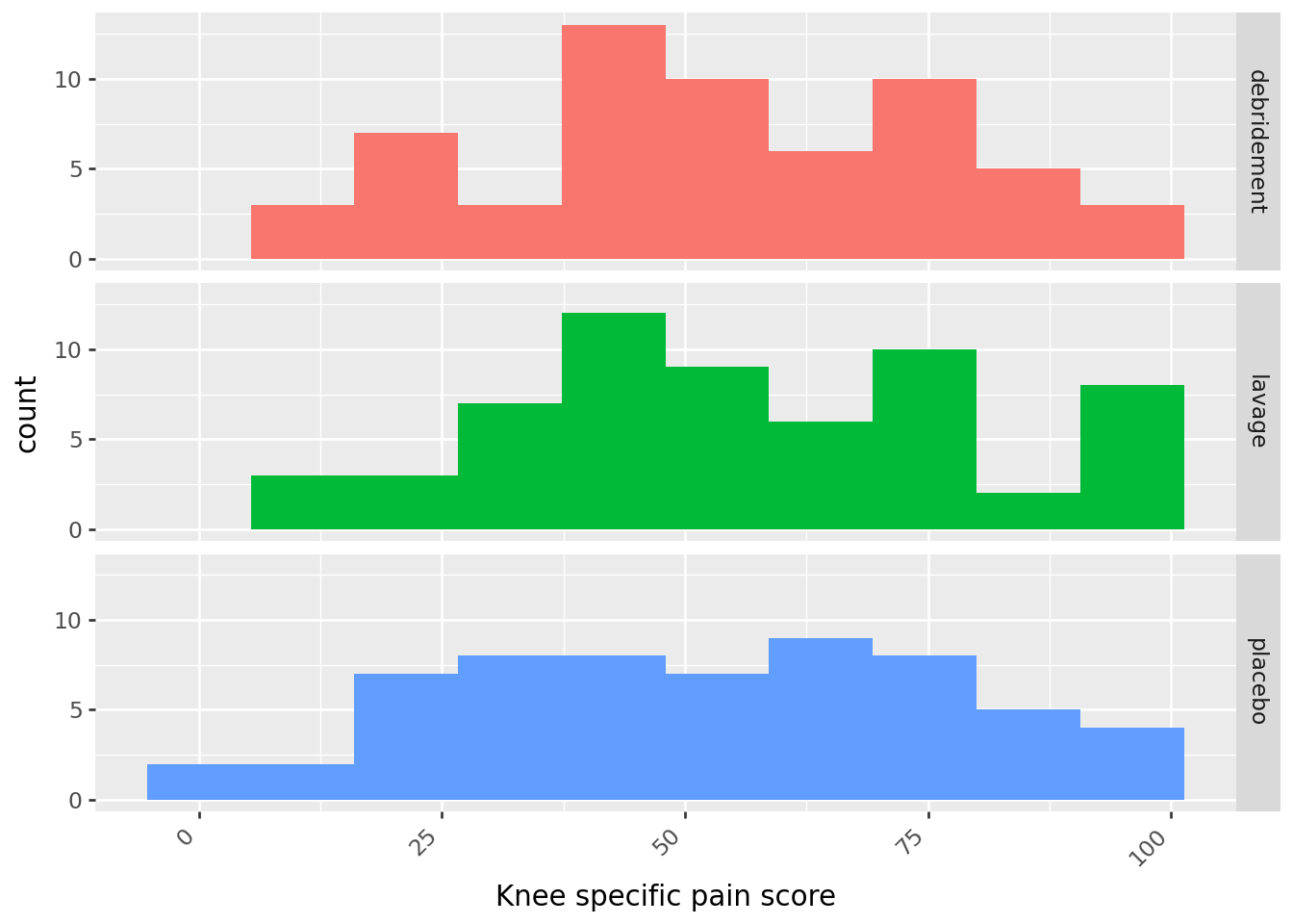
Example 28.1 When medical therapy fails to relieve the pain of osteoarthritis of the knee, arthroscopic lavage or debridement is often recommended. More than 650,000 such procedures are performed each year at a cost of roughly $5,000 each. A recent double blind experiment investigated the effectiveness of these procedures1. 180 subjects with osteoarthritis of the knee were randomly assigned to receive one of three treatments: arthroscopic lavage (which involved flushing the knee joint with fluid), arthroscopic debridement (which involved both lavage and shaving of cartilage and removal of debris), and placebo surgery (which involved incisions in the knee, but no insertion of instruments). Various outcomes were measured; the summaries below summarize scores two years after the procedure on a knee-specific pain scale (0-100, with with higher scores indicating more severe pain). Does any procedure tend to result in better pain scores on average?
- State the null and alternative hypotheses (in words is fine).
- The summarizes the sample data. Do you think there will be any evidence to reject the null hypothesis?
- Suggest a statistic which could be used to perform a hypothesis test.
Example 28.2 Consider the following plots, which are all on the same scale. (This example just illustrates some general ideas so the context isn’t important, but the data relate to a study on different types of diet plans (Atkins, etc) and weight loss.) Plot A displays the study data. Plots B and C show hypothetical data sets with the same group sizes as in Plot A. Group means are indicated by the colored vertical lines.
- The SD for each group in Plot B equals the SD for the corresponding group in Plot A.
- The mean for each group in Plot C equals the mean for the corresponding group in Plot B.
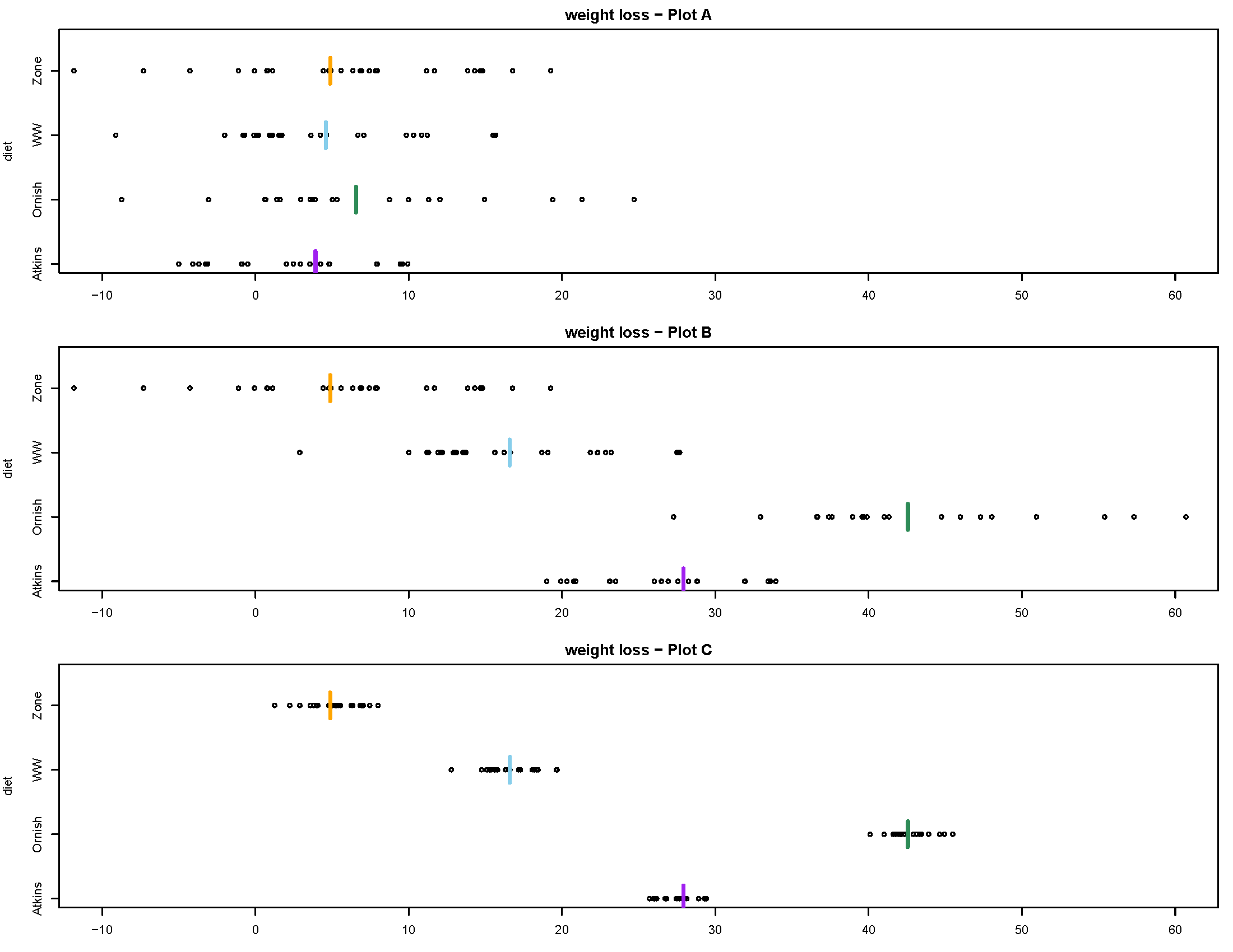
Rank the plots in order from weakest to strongest evidence to reject the null hypothesis of no difference in means between treatments. That is, rank the plots in order from largest to smallest p-value.
Compare plots A and B.
- The variability between groups in Plot B is (choose one: >, <, =) the variability between groups in Plot A.
- The variability within groups in Plot B is (choose one: >, <, =) the variability within groups in Plot A.
Compare plots B and C.
- The variability between groups in Plot C is (choose one: >, <, =) the variability between groups in Plot B.
- The variability within groups in Plot C is (choose one: >, <, =) the variability within groups in Plot B.
Rank the plots in order from smallest to largest \(F\) statistic.
- Example 28.2 illustrates the idea behind the \(F\) statistic: we reject the null hypothesis of no difference in means between groups/populations/treatments if the observed variability between groups is large relative to the observed variability within groups.
- Roughly, we reject the null hypothesis if the ratio \[ \frac{\text{variability between groups}}{\text{variability within groups}} \] is large enough. This idea is known as analysis of variance (ANOVA).
- The name ANOVA refers to what we are doing, and not why we are doing it.
- Remember, we are analyzing the variance to make a conclusion about the means
- The \(F\) statistic quantifies the above ratio. The larger the value of the \(F\) statistic the stronger the evidence to reject the null hypothesis (of no difference) in favor of the alternative hypothesis (of some difference). That is, the largest the \(F\) statistic the smaller the p-value.
Example 28.3 Continuing Example 28.1. The computation of the \(F\) statistic is full of technical details. We will only do a rough hand computation which illustrates the main ideas, but we’ll usually rely on software to compute it. The computation is somewhat simplified when the sample size is the same for each explanatory variable group.
What statistic can be used to measure the variability within the Debridement group? Lavage? Placebo? How could you combine these numbers to to measure, in a single number, variability within groups?
If the null hypothesis is true, what would you expect about the group means? What statistic can be used to measure the variability between groups?
Regardless of whether or not the null hypothesis is true, which of the values from the previous parts would you expect to be larger? Why?
So far, we have used the group means and group SDs in our calculations. What other feature of the groups do you think will influence the results? How?
Compute the \(F\) statistic.
What value would you expect \(F\) to be if the null hypothesis is true? Specify in detail how you could use simulation to approximate the null distribution of the \(F\) statistic.
Figure 28.1 displays results from an applet used to run 10000 repetitions of the simulation. How could you use the simulation results to approximate the p-value? Could you use the empirical rule for Normal distributions?
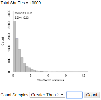
Figure 28.1: Permutation null distribution of \(F\) statistic for Example 28.1. State a conclusion in context. Are the results “significant”?
If we were to compute a series of pairwise confidence intervals for the difference in group means — Debridement \(-\) Lavage, Debridement \(-\) Placebo, Lavage \(-\) Placebo — what value would each of the confidence intervals contain? Why?
Hypothesis test for comparing multiple means: “One-way ANOVA \(F\) test”
- Situation: \(N\) observations of numerical response variable; categorical explanatory variable with \(g\) groups
- Parameters: \(\mu_j\)’s are the population/process/treatment response means; \(\sigma\) is the common group SD of responses
- Goal: test for any differences in means
- The null hypothesis is \(H_0: \mu_1=\cdots=\mu_g\) (“no difference” or “no treatment effect”)
- The alternative hypothesis is not \(H_0\); that is, there is some difference in means between groups, \(H_1: \mu_j\neq \mu_k \text{ for some } j\neq k\)
- Test statistic: one-way ANOVA \(F\) statistic \[ F = \frac{\sum_{j=1}^g n_j\left(\bar{x}_j - \bar{x}\right)^2/(g-1)}{\sum_{j=1}^g (n_j-1)s^2_j/(N-g)} \]
- The p-value is the probability of observing a value at least as large as the observed \(F\) based on an \(F\) distribution with \(g-1\) degrees of freedom in the numerator and \(N-g\) degrees of freedom in the denominator
- Assumptions:
- Either:
- The data are obtained through multiple unbiased and independent random samples from large populations
- Or from one unbiased random sample which can be classified into multiple groups, and the groups can be considered independent of each other.
- The data are obtained from an experiment in which subjects were to two treatments.
- The data are obtained through multiple unbiased and independent random samples from large populations
- No bias in data collection
- Comparing means is an appropriate analysis
- Equal variance: True SD of responses is same, \(\sigma\), for each population/process/treatment.
- Typically satisfied through random assignment.
- Might not be satisfied if the data are sampled from different populations/processes.
- One rule of thumb is that the largest observed sample SD should be no more than twice the smallest.
- Either:
- Special case: when the group size \(n\) is the same for all \(g\) groups is \[\begin{align*} F & = \frac{\text{group size} \times \text{variance of group means}}{\text{mean of group variances}}\\ & = \frac{n\sum_{j=1}^g \left(\bar{x}_j-\bar{x}\right)^2/(g-1)}{\sum_{j=1}^g s_j^2/g } \end{align*}\]
- The calculations are traditionally summarized in an ANOVA table
| Source | df | SS (Sum of squares) | MS (Mean Square) | \(F\) |
|---|---|---|---|---|
| Between groups (a.k.a. “treament”) | \(g-1\) | SS(between) = \(\sum_{j=1}^g n_j\left(\bar{x}_j - \bar{x}\right)^2\) | \(\frac{\text{SS(between)}}{g-1}\) | \(\frac{\text{MS(between)}}{\text{MS(within)}}\) |
| Within groups (a.k.a. “error”) | \(N-g\) | SS(within) = \(\sum_{j=1}^g (n_j-1)s^2_j\) | \(\frac{\text{SS(within)}}{N-g}\) | |
| Total | \(N-1\) | (SS(between) + SS(within)) = \(\sum_{i=1}^N\left(x_{i} - \bar{x}\right)^2\) |
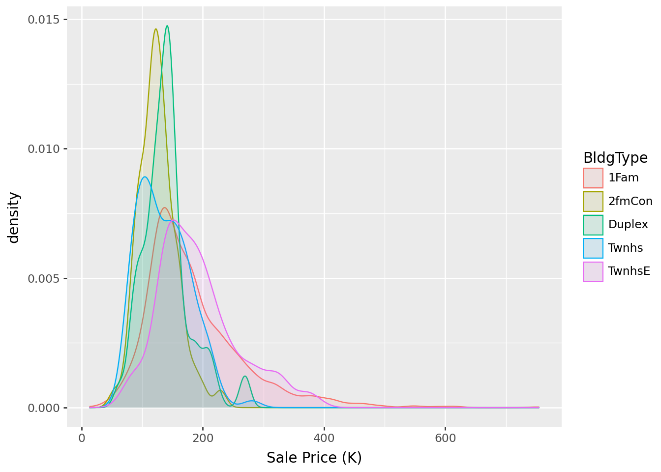
Example 28.4 Continuing with the Ames housing data set. Now suppose we want to compare sale price of homes by building type: single-family (1Fam), two-family (2fmCon), duplex, townhouse end unit (TwnhsE), townhouse inside unit (Twnhs).
| count | mean | std | min | 25% | 50% | 75% | max | |
|---|---|---|---|---|---|---|---|---|
| BldgType | ||||||||
| 1Fam | 2425.0 | 184.812041 | 82.821802 | 12.789 | 130.0000 | 165.000 | 220.000 | 755.00 |
| 2fmCon | 62.0 | 125.581710 | 31.089240 | 55.000 | 106.5625 | 122.250 | 140.000 | 228.95 |
| Duplex | 109.0 | 139.808936 | 39.498974 | 61.500 | 118.8580 | 136.905 | 153.337 | 269.50 |
| Twnhs | 101.0 | 135.934059 | 41.938931 | 73.000 | 100.5000 | 130.000 | 170.000 | 280.75 |
| TwnhsE | 233.0 | 192.311914 | 66.191738 | 71.000 | 145.0000 | 180.000 | 222.000 | 392.50 |
                   sum_sq      df          F        PR(>F)
C(BldgType)  6.454111e+05     4.0  26.151358  2.475923e-21
Residual 1.804713e+07 2925.0 NaN NaN- Table 28.1 is the ANOVA table. State the conclusion of the ANOVA \(F\) test in context.
- Consider the conclusion of the \(F\) test. What are some natural follow-up questions? How might you use the data to answer them?
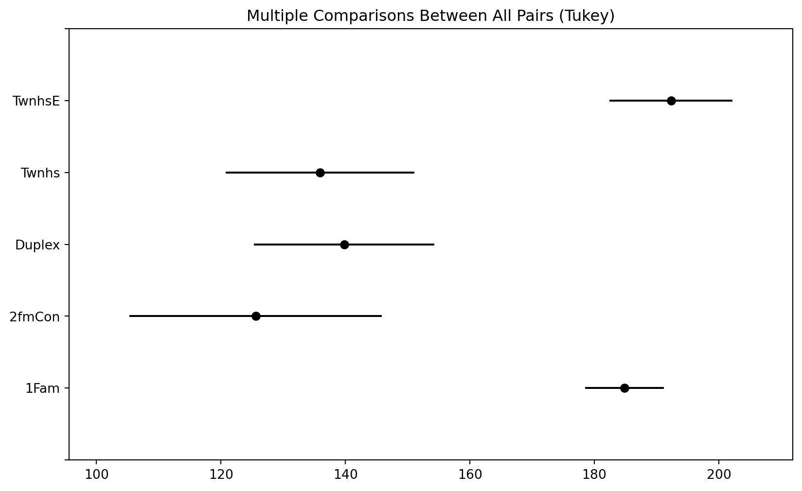
- Table 28.2 contains the results of Tukey pairwise 95% confidence intervals. Interpret these intervals in context.
 Multiple Comparison of Means - Tukey HSD, FWER=0.05
======================================================
group1 group2 meandiff p-adj   lower    upper   reject
------------------------------------------------------
  1Fam 2fmCon -59.2303    0.0 -86.8048 -31.6559   True
  1Fam Duplex -45.0031    0.0 -65.9952 -24.0111   True
  1Fam  Twnhs  -48.878    0.0 -70.6511 -27.1049   True
  1Fam TwnhsE   7.4999 0.6328  -7.2051  22.2048  False
2fmCon Duplex  14.2272  0.786 -19.8771  48.3316  False
2fmCon  Twnhs  10.3523 0.9255 -24.2382  44.9429  False
2fmCon TwnhsE  66.7302    0.0  36.0924   97.368   True
Duplex  Twnhs  -3.8749 0.9965 -33.4861  25.7363  False
Duplex TwnhsE   52.503    0.0  27.6234  77.3825   True
 Twnhs TwnhsE  56.3779    0.0  30.8358  81.9199   True
------------------------------------------------------
- Rejecting the null hypothesis based on an \(F\) statistic only tells you that “the mean for at least one of the treatments (populations) is not the same as the mean for at least one of the other treatments (populations)”.
- The natural follow-up questions are: which treatment (population) means differ? and by how much?
- One approach when you have rejected the null hypothesis is to calculate — using software — all pairwise confidence intervals. In particular, which intervals do not contain zero?
- When computing multiple confidence intervals, the multiple (\(z^*\) or \(t^*\)) should be increased2 to account for the issue of multiple comparisons (recall Example 24.5 and related notes).
- Tukey’s method is a widely used method for constructing simultaneous confidence intervals for all pairwise comparisons of means. The confidence intervals computed using Tukey’s method already contain an adjustment to account for multiple comparisons.
There are several ways to do this. The simplest is a Bonferroni adjustment, which splits the error rate evenly across all intervals. For example, for simultaneous 95% confidence in 10 intervals (i.e. a total error rate of 0.05), use the \(t^*\) factor for 99.5% confidence (\(0.995 = 1-0.05/10\)), \(t^*= 2.8\), instead of 2 when computing the intervals. But the Tukey method is more widely used when comparing means.↩︎