| count | mean | std | min | 25% | 50% | 75% | max | |
|---|---|---|---|---|---|---|---|---|
| SingleFamily | ||||||||
| False | 505.0 | 161.511398 | 60.394023 | 55.000 | 120.0 | 147.4 | 190.0 | 392.5 |
| True | 2425.0 | 184.812041 | 82.821802 | 12.789 | 130.0 | 165.0 | 220.0 | 755.0 |
26 Null Hypothesis Testing
- Statisticians view conjectures about a population as competing hypotheses. These hypotheses usually constitute claims about the values of certain parameters.
- A statistical (null) hypothesis test consists of using data to make a decision regarding two explanations (hypotheses).
- The null hypothesis, denoted \(H_0\), represents the “status quo/no difference/no effect/no association” hypothesis.
- If the null hypothesis is true then any observed difference/effect/association is just due to “random chance” resulting from natural sampling variability
- The alternative hypothesis, denoted \(H_a\) (or \(H_1\)), typically corresponds to what the researchers are hoping to gather evidence to support, and thus is a statement in line with the research conjecture
- A statistical hypothesis test assesses if the data provide evidence to rule out the “random chance” explanation (which corresponds to the null hypothesis) in favor of the explanation provided by the research conjecture (alternative hypothesis).
- The null hypothesis is often of the form \[H_0: \text{parameter} = \text{hypothesized value}\] where the hypothesized value is a specific number determined by the research question (often 0 for “no difference”).
- The alternative hypotheses is often of one of the following forms \[\begin{aligned} \text{Case 1a:}\quad H_a: \text{parameter} &> \text{hypothesized value}\\ \text{Case 1b:}\quad H_a: \text{parameter} &< \text{hypothesized value}\\ \text{Case 2:}\quad H_a: \text{parameter} &\neq \text{hypothesized value (``two-sided'')} \end{aligned}\] Which of the three cases above is appropriate is determined by the research conjecture. When in doubt, use a two-sided (\(\neq\)) alternative.
Example 26.1 Did the New England Patriots deliberately deflate footballs in an NFL playoff game against the Indianapolis Colts on January 18, 2015? The following table1 summarizes the decrease in air pressure (psi), from pre-game to halftime, for the footballs from each team that were checked at halftime by officials.
| Team | Deflation (psi) | Size | Mean | SD | ||||||||||
|---|---|---|---|---|---|---|---|---|---|---|---|---|---|---|
| Patriots | 1.00 | 1.65 | 1.35 | 1.80 | 1.40 | 0.90 | 0.65 | 1.40 | 1.55 | 2.00 | 1.60 | 11 | 1.391 | 0.402 |
| Colts | 0.30 | 0.25 | 0.50 | 0.45 | 4 | 0.375 | 0.119 |
- Compute the observed difference in sample means.
- If there were no difference between the Patriots and the Colts footballs, what would you expect the difference in sample means to be? Is the fact that we observed another value necessarily evidence that the Patriots footballs tended to deflate more than the Colts?
- Suppose we want to assess if it is plausible that the Patriots didn’t interfere with the footballs, and the observed difference in sample means is just due to chance variability. Specify how the “null distribution” of the statistic could be simulated with cards. Note: this is NOT bootstrapping; how is it different?
- Use cards to perform one repetition of the above simulation, record the results here, and compute the appropriate difference in means.
| Team | Deflation (psi) | Size | Mean | SD | ||||||||||
|---|---|---|---|---|---|---|---|---|---|---|---|---|---|---|
| Patriots | 11 | |||||||||||||
| Colts | X | X | X | X | X | X | 4 |
- The following plot displays results from an applet used to run 10000 repetitions of the simulation (the plot on the left displays the results from just the first 100 repetitions). Estimate the probability of observing a difference in sample means as extreme as the observed difference just by chance if there were no real difference between the Patriots and Colts footballs.
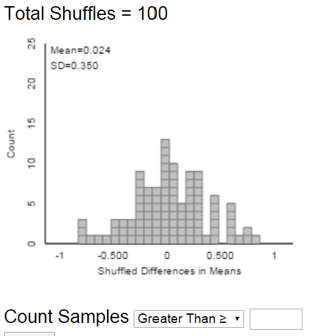
- Is it plausible that the observed difference in means is just due to random chance? To support your answer, interpret the probability from the previous part in context.
- To assess the plausibility of the “random chance” explanation for the observed result — corresponding to the null hypothesis being true — we need to know the pattern of sampling variability of the statistic that would be expected just due to random chance if the null hypothesis were true. This is called the null distribution of the statistic.
- If the actual observed value of the statistic is not consistent with this pattern, then we have convincing evidence that the results did not occur by random chance alone, and we have evidence to reject the null hypothesis
- The (simulated) null distribution provides a picture of what typical values of the statistic would be expected just by random chance alone if the null hypothesis were true.
- The question is then: how surprising is the result we actually observed from the perspective of the null distribution? If the result would be very surprising, then “random chance” is not a plausible explanation for the observed result.
- This gives us evidence to rule out a “random chance” explanation like in favor of a “research conjecture” explanation.
- In other words, the more surprising the observed result would be just due to random chance, the stronger the evidence to reject the null hypothesis in favor of the alternative hypothesis.
- We quantify “how surprising” with a p-value.
- The p-value is the probability of observing a value at least as extreme as the value actually observed, when the null hypothesis is true.
- The p-value can be estimated by the proportion (out of the total number of repetitions) of values in the simulated null distribution that are at least as extreme as the actual observed value of the statistic.
- Which tail(s) constitutes “at least as extreme" is determined by the form of the alternative hypothesis
- The smaller the p-value — that is, the closer the p-value is to 0 — the less plausible it is that the observed result occurred just by random chance alone.
- Thus, the smaller the p-value the stronger the evidence to reject the null hypothesis in favor of the alternative hypothesis.
- If the observed results provide strong evidence that the data did not arise by random chance alone — that is, when the p-value is small — then there is evidence of a statistical difference.
- How small is a small p-value? You should think of a sliding scale: the closer the p-value gets to 0 the stronger the evidence to reject the null hypothesis in favor of the alternative. Some guidelines are below, but these should not be followed too strictly (especially when performing many hypothesis tests simultaneously):
- Do NOT rely strictly on arbitrary thresholds like p-value \(<\) 0.05.
| p-value | Evidence to reject the null hypothesis? |
|---|---|
| Above 0.10 | Little to no evidence |
| Between 0.01 and 0.10 | Weak evidence |
| Between 0.001 and 0.01 | Moderate evidence |
| Between 0.0001 and 0.001 | Strong evidence |
| Less than 0.0001 | Very strong evidence |
Example 26.2 Carrying a heavy backpack can cause chronic shoulder, neck, and back pain. A common recommendation is that a daily backpack should not weigh more than 10 percent of the wearer’s body weight. Do Cal Poly students follow this recommendation? That is, do the backpacks of Cal Poly students weigh, on average, less than 10% of their bodyweight? In a random sample of 100 Cal Poly students the sample mean backpack weight as percent of bodyweight is 7.71 percent with sample standard deviation 0.366 percent.
- Identify the main parameter of interest with both words and an appropriate symbol.
- Translate the research question into a hypothesis testing problem by specifying, with both words and appropriate symbols, the null hypothesis and the alternative hypothesis.
- Identify the null distribution of sample means. (You might need to make some assumptions.)
- Compute the p-value.
- Interpret the p-value in context.
- Does the p-value provide evidence that backpacks of CalPoly students weigh, on average, less than 10% of their bodyweight? Explain.
- Does the p-value provide evidence that backpacks of CalPoly students weigh, on average, much less than 10% of their bodyweight? Explain.
- How could we address the question in the previous part?
- Do Cal Poly students follow the 10% recommendation? Is the analysis above the only way to address this question? Can you suggest another?
One-sample \(t\) test
- Situation: question concerns a single numerical variable of interest
- Parameter: \(\mu\) is the population mean (i.e. the mean value of the variable over all units in the population)
- Goal: assess the plausibility of a claim about \(\mu\) regarding a hypothesized value \(\mu_0\)
- The null hypothesis is \(H_0: \mu= \mu_0\)
- The alternative hypothesis is one of \(H_a: \mu >\mu_0\), \(H_a: \mu<\mu_0\), or \(H_a: \mu\neq \mu_0\)
- When in doubt, use a two-sided alternative and a two-tailed p-value.
- Statistics: \(\bar{x}\) is the sample mean; \(s\) is the sample standard deviation
- Test statistic: the standardized value of \(\bar{x}\), where
- the mean is computed assuming the null hypothesis, \(H_0: \mu=\mu_0\), is true, and
- the unknown SD (\(\sigma/\sqrt{n}\)) is estimated with the standard error \(s/\sqrt{n}\) \[ t = \frac{\text{observed}-\text{hypothesized}}{\text{SE}} = \frac{\bar{x}-\mu_0}{s/\sqrt{n}} \]
- The p-value is the probability of observing a value at least as extreme as \(t\), in the tail direction indicated by the alternative hypothesis, for the \(t\)-distribution with \(n-1\) degrees of freedom.
- In almost all situations encountered in practice you can use the usual empirical rule for Normal distributions
- Assumptions:
- Simple random sample from a large population, that is, independent observations
- No bias in data collection
- Population mean is the parameter you want to estimate
Example 26.3 Continuing with the Ames housing data set. Now suppose we want to compare sale prices of single family homes with other homes (including condos, townhouses, etc). In particular, do single family homes tend to have higher sale prices on average than other homes?
The table below summarizes the sample data.
- Explain how you could use simulation to approximate the p-value.
- Use the sample data to conduct by hand an appropriate hypothesis test.
- Write a clearly worded sentence interpreting the p-value in context.
- Does the p-value provide evidence that single family homes tend to have higher sale prices on average than other homes? Explain.
- Does the p-value provide evidence that single family homes tend to have much higher sale prices on average than other homes? Explain.
- How could we address the question in the previous part?
Two-sample \(t\) test for a difference in population (or treatment) means.
- Situation: binary explanatory variable (population/treatment 1, 2) and numerical response variable
- Parameter: \(\mu_1-\mu_2\) is the difference in population means (treatment means)
- Goal: assess the strength of the evidence against the “no difference” or “no treatment effect” hypothesis
- The null hypothesis is \(H_0: \mu_1-\mu_2=0\)
- The alternative hypothesis is one of \(H_a: \mu_1-\mu_2>0\), \(H_a: \mu_1-\mu_2<0\), or \(H_a: \mu_1-\mu_2\neq0\)
- When in doubt, use a two-sided alternative and a two-tailed p-value.
- Statistic: \(\bar{x}_1-\bar{x}_2\) is the difference in sample means for samples (groups) of size \(n_1, n_2\)
- The SE of the difference in sample means is \[ \textrm{SE}(\bar{x}_1-\bar{x}_2) = \sqrt{\frac{s_1^2}{n_1}+\frac{s_2^2}{n_2}} = \sqrt{\textrm{SE}^2(\bar{x}_1)+\textrm{SE}^2(\bar{x}_2)} \]
- Test statistic: \[ t = \frac{\text{observed}-\text{hypothesized}}{\text{SE}} = \frac{\bar{x}_1-\bar{x}_2-0}{\sqrt{\frac{s_1^2}{n_1}+\frac{s_2^2}{n_2}}} \]
- The p-value is the probability of observing a value at least as extreme as \(t\), in the tail direction indicated by the alternative hypothesis, for the \(t\)-distribution with (complicated) degrees of freedom.
- In almost all situations encountered in practice you can use the usual empirical rule for Normal distributions
- Assumptions:
- Either
- The data are obtained through two unbiased and independent random samples from large populations
- Or from one unbiased random sample which is classified according to two variables, and the two groups can be considered independent of each other.
- The data are obtained from an experiment in which subjects were randomly assigned to two treatments.
- The data are obtained through two unbiased and independent random samples from large populations
- No bias in data collection
- Difference in population means is the parameter you want to estimate
- Either
- The \(t\) procedures for population means are valid as long as the sample size is large enough, regardless of the shape of the population distribution.
- However, if the population distributions are highly skewed, then the population medians might be more appropriate parameters to consider as measures of center.
- Which is more appropriate, the population means or the population medians, depends on the purpose for the inference.
- Also remember that sample means and SDs, and hence \(t\) procedures, are sensitive to outliers and extreme values.
Example 26.4 In Example 26.2 and Example 26.3 we both performed a null hypothesis test and computed a confidence interval. Discuss the advantages and disadvantages of each approach.
- Confidence intervals and hypothesis tests are commonly used in conjunction, but they address different questions
- Hypothesis test: How strong is the evidence that there is a difference (or association or effect)?
- Confidence interval: How large is the difference (or association or effect)?
- A confidence interval
- provides a range of plausible values
- but the cut-off between plausible and implausible is arbitrary (e.g. 95% confidence corresponds to \(\alpha=0.05\))
- But be especially careful about interpreting confidence when conducting multiple confidence intervals.
- A null hypothesis test
- Considers the plausibility of only a single hypothesized value
- But provides a precise measure — the p-value — of the plausibility of the particular hypothesized value in light of the observed data
- But be especially careful about interpreting p-values when conducting multiple hypothesis tests.